ANSYS Workbench 19.2

Editor’s Note: Tony Abbey provides live e-Learning courses, FEA consulting and mentoring. Contact tony@fetraining.com for details, or visit his website.

ANSYS Workbench pulls together the company’s traditional solver and its pre- and post-processing functions into a single integrated platform. Geometry creation and manipulation is also fully linked into Workbench. Project control is centralized in a visual drag-and-drop Project Schematic graphics area. Project control can include analysis chaining or linking within a discipline. It allows re-use of workflow elements, such as materials, geometry or analysis setup. In addition, multi-disciplines can be linked via the Schematic window.

I have been using the shallow roof model shown in Fig. 1 in my non-linear training classes for a while.

It represents a structure that is initially stable under loading, but then with further loading, transitions or “snaps” to a new stable configuration. This behavior is shown in Fig. 2.

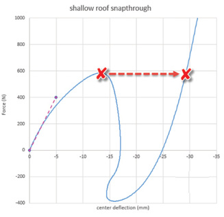
The full snap-through follows the blue line and shows unloading, reverse loading and reverse deflection. The red line shows the overall “jump” from one configuration to another. The debate is in how the transition occurs.

There are many real-world examples of snap-through, such as the lid of an oil drum with an internal vapor pressure, mechanical switch systems or metal “clickers” for dog training. It has been used as a benchmark for many years.

As I mentioned in a previous DE article (January 2018, “Demos and Benchmarks”), it is a typical example of a benchmark that is numerically challenging but is flawed, practically speaking. The reason it is flawed is that static stability is required at each load step in the benchmark. This is impractical once snap-through has started. This implies counterbalancing forces and reversal of motion at the center point during the snap-through. The three classic types of loading are:

1. force-controlled loading that applies a monotonically increasing force at the center point;

2. displacement-controlled loading that is enforced at the center point; and

3. arc length displacement-controlled loading that permits reverse displacement (“snap-back”).

The discussion was based on the fact that none of these loadings is realistic. The plate will tend to move away from whatever is loading the central point during snap-through and the snap-through will be dynamic in nature.

I used ANSYS to explore the physics of this benchmark more deeply, in particular, looking at contact and dynamic loading.

User Interface

On launching ANSYS Workbench, the main user interface appears as shown in Fig. 3. In the main Toolbox menu, we can see a wide range of Analysis Systems available, based on the physics applications purchased. In addition to the mechanical-based solutions, this can embrace computational fluid dynamics (CFD), thermal, electromagnetic and others.

I have selected the Static Structural Analysis System. The corresponding workflow is shown in the Project Schematic graphics window. I will be using both Static Structural (which includes non-linear analysis) and Transient Structural.

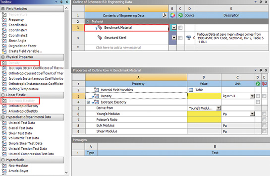
Each step of the workflow is completed in turn, and a checkmark appears when the data is acceptable to ANSYS Workbench. Fig. 3 shows I have a checkmark against the Engineering Data cell, but this is based on automatic loading of a default material. To change this, double-click on the Engineering Data cell and the Material Input forms appear as shown in Fig. 4.

The shallow roof benchmark material is assumed to be a type of polyimide, based on the defined material properties. I have created a material called “benchmark” by clicking on the Isotropic Elasticity and Density options. The yellow highlighted regions show where to input the data. I have selected project units to be Kg, m, S. Young’s Modulus is 3.1E9 N/m^2 (Pa), Poisson’s ratio is 0.3, and I have used a typical polyimide value of 1,430 kg/m^3 for density (this is not defined in the benchmark).

Many other material models and physical properties can be defined in Workbench, including Plasticity, Hyperelastic, Viscoelastic, Creep and Fracture Criteria options. You can also define custom material models.

Model Setup

The next stage in the workflow is to define the geometry that underpins the finite element analysis (FEA) model. In my case I elected to import the roof geometry as a SolidWorks part. Importing within the Geometry cell opens the SpaceClaim CAD tool in a separate window.

SpaceClaim is a sophisticated Direct CAD modeling tool that permits setup and fast redesign of components. I have not explored this tool in any depth, as I am focusing on the FEA capabilities of Workbench. DesignModeler, an alternative parametric geometry modeler, is also available. ANSYS documentation suggests using the latter tool for manipulating existing geometry and SpaceClaim for creating geometry from scratch.

I prepared the geometry in SolidWorks by creating a mid-surface object of the roof segment and an additional sketch that contains construction curves. The latter are imported by SpaceClaim as curves and can then be imprinted onto the surface to provide subdivisions for meshing and loading point location.

Alternatively, if you are familiar with SpaceClaim, the geometry can be created and prepared very quickly within that environment.

The Geometry workflow item is now automatically checked in the Workbench schematic and the Model cell is double-clicked to launch ANSYS Mechanical, as shown in Fig. 5.

Fig. 5 shows the central region, controlled by a Face Sizing mesh control, set to 5 mm. The default mesh is 22.45 mm. There are extensive mesh controls and mesh quality checking within the software. The thickness of the surface geometry is defined as 6.35 mm, and this is inherited by the shell elements. The material property is also allocated to the geometry and inherited by the mesh.

The load is set up as a point force applied to the central geometric vertex. The edge constraints are set up as simply supported on the two straight edges. Arbitrary constraint degrees of freedom (DOF) are selected by using the Displacement option and setting appropriate DOF to zero.

The Mechanical Interface allows both linear and non-linear, depending on the physics defined. The non-linear settings I used are shown in Fig. 6.

I have turned on the Large Deflection option. This allows the geometric non-linearity inherent in this problem to be modeled. I have also used Time to control the nonlinear steps used in the analysis. The default is to use Substeps.

In a static solution, time has no meaning, so an arbitrary duration of 1 second represents 100% loading. The initial time step is 0.01 seconds (implying 100 steps). The minimum is set as a further factor of 1/10 of this (0.001 seconds) and the maximum is set as 0.05 seconds.

ANSYS highlights any inconsistent values in yellow, which is useful for checking. The nonlinear iteration strategy is set using the defaults for the Newton-Raphson method. ANSYS will control the time steps, adapting from the initial value I have set. The actual values and strategy you will use can vary considerably in any analysis and it is recommended that numerical testing is carried out to get a feel for the applicability of these settings.

The required output results are defined prior to the analysis. I chose Total Displacement and von Mises Stress. I also used a Data Probe to find the vertical displacement at the center vertex and to sum the reaction forces at the simply supported edges. Grouping reaction forces by constraint label or entity is useful.

Analysis Results

The results are investigated once I launch the analysis. The roof structure exhibits a snap-through at around 12 mm of deflection. The reaction force versus center deflection plot shown in Fig. 7 shows the classic jump of the force-controlled solution, across the snap-through.

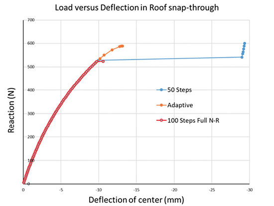
With a force-controlled loading, as carried out here, the loading can only ever increase, so the only valid solutions are found on the other side of the “jump” as the structure reaches the next stable configuration. At some point, the stiffness of the structure drops to zero just prior to the snap-through (the load deflection curve is horizontal). If the solution gets too close to that point, then it cannot converge to an equilibrium state and the analysis stops.

My initial settings are too “clever” in a sense, as they will allow the time step to adapt and get very close to the zero-stiffness point. I have repeated the analysis a few times with a manual time-step to get a solution just prior to snap-through, which can then jump to the next stable solution and bypass the snap-through. A step size of 0.02 seconds (50 steps) achieves this, as shown in Fig. 7.

ANSYS Workbench allows fast redefinition of the non-linear controls. In addition, a straightforward restart capability is available. In a complex model this would allow a converged point at, say, 10 mm to be established and reused. Non-linear settings could be explored beyond this, without wasting resources up to the 10 mm point.

The summary text output from the ANSYS solver can be monitored within the Workbench environment during the analysis. This can be very useful to understand the implications of non-linear settings on non-linear convergence and iteration strategy.

The probe results (displacement and reaction force) are automatically available as xy plots and can be easily stepped through. Full contour plots can be retrieved at critical times identified from the xy plots.

I have plotted the compound results shown in Fig. 7 by using Excel; however, a Workbench Chart facility allows tabling and plotting of responses against each other, within the Workbench environment. The resulting Chart object can be labeled and used as a container for plots and tabular results in subsequent analysis, with easy export to Excel.

The Total Displacement option contains results for the complete analysis and snapshots are shown in Fig. 8. The displacement history can be animated directly from the graphics window. Stepping to critical points is carried out with incremental controls.

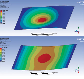
The initial configuration is shown in Fig. 8(a) with a central deflection of 9.4 mm. The final stable configuration, after snap-through, is shown in Fig. 8(b). The central deformation is 31.5 mm. The deformation mode is totally different from the initial configuration, with overall bending behavior in addition to the center “dimple”-shaped deflection.

A Second Analysis Type

The next task was to replace the central force with a displacement control. I renamed this as “Displacement control,” and the Project Schematic window shows the automatic association made between Engineering Data, Geometry and Model. The next change I need to make is in Setup. Double-clicking on this cell reopened ANSYS Mechanical and I replaced the center point load with an enforced displacement of 30 mm. The reaction force versus central deflection response now appears in Fig. 9.

Various settings are shown in the figure, with the 100 steps manual solution coming closest to the theoretical vertical drop as the snap-through response tries to reverse the deflection. The deflection-controlled loading cannot “snap back” beyond the vertical. Note that the automatic method can’t adapt quickly enough to the rapidly changing stiffness. This is typical of all solvers I have used, and emphasizes the need for user exploration. ANSYS Workbench makes numerical experimentation straightforward to carry out by using readily accessible parameter controls.

The solutions all overlay the force-controlled solution up to the limit load (zero stiffness) and transition to the same secondary stable solution after snap-through.

To achieve the classic snap-back solution, which allows the displacement to reverse, an Arc-Length method is required. This is not supported directly in ANSYS Workbench but is available in ANSYS and can be accessed from Workbench by using the APDL (ANSYS Parametric Design Language). Inserting a Command opens the interface for direct entry of APDL commands.

Setting up Contact

As described earlier, it was thought that a contact-controlled loading would be realistic, so I took the opportunity to set this up in ANSYS Workbench.

I opened a new Structural Analysis workflow in the Project Schematic window and named this as Contact Control. Only the material was reused, and I dragged a link from the corresponding Material cell in the previous analysis to inherit this data.

A bullet-shaped impactor was set up in SolidWorks geometry and imported into SpaceClaim. The face of the bullet and the plate were imprinted in SpaceClaim to improve the mesh and provide probe points for displacement results.

I used a manual selection technique, but automatic detection is available. The two regions are described as Body and Target in Workbench and window panes are spawned automatically, making region picking straightforward.

The bullet is displacement controlled and made of steel. In the subsequent analysis I only used the tip region, as the body was redundant. For a more complex model I could have used a rigid material, with a master displacement control over contact segments, to avoid wasting resources on a deformable bullet.

Controls are set to use the top surface of the shell as the contact surface—this is important in thin shell contact modeling to avoid the mid-surface beginning used, with subsequent errors in contact geometry.

Local mesh controls on the plate and bullet surface were useful in improving contact accuracy and convergence. A spherical mesh refinement zone can be visualized and defined around a vertex. This was used at the contact center points. After some experimentation, non-symmetric contact using the Augmented Lagrangian Contact method gave the best results.

Contact Results

In this setup, the plate snaps away from bullet as a result of the snap-through behavior. This separation is more realistic than an entrained displacement. ANSYS reports loss of contact in a message window, as the analysis progresses. The bullet then catches up with the plate and re-establishes contact. Again, the ANSYS live message is useful to warn users that the contact stiffness has changed abruptly. Fig. 10 shows a series of reaction force versus central displacement plots for this setup.

The initial result was with a 50 mm radius bullet and showed a lower snap-through load than the displacement control. Changing to a 25 mm radius bullet showed a match with the previous displacement control, which is also shown in Fig. 10.

The reaction force now drops to zero during the snap-through. Without contact, there can be no load transfer. Relative movement of the bullet and plate without contact is a challenging period for stability in a static solution. I found using the option to use system-defined “soft springs” to be helpful in stabilizing the solution here.

I used SpaceClaim to sharpen the bullet from 50 mm to 25 mm radius. This is a basic example of the geometry control that can be carried out in Workbench using the direct “push/pull” and other morphing methods. The radius of the arc becomes the design driver in this parametric analysis study.

Dynamic Results

Using contact control, the “gap” between snap-though pulling the plate away from the bullet and the bullet catching up with the plate is tough for static equilibrium to represent. In practice, inertia effects will play an important role.

Hence the next stage is to set up a transient nonlinear dynamic analysis in Workbench. A Transient Analysis system is chosen from the main Workbench Toolbox and placed on the Project Schematic. The Engineering Data, Geometry and Model cells can be linked to the previous analysis so that this data is inherited. All that is required now is to set up the time dependency of the displacement control and the transient analysis time step controls.

I used 35 mm deflection applied over 0.1 second. That represents about 1.26 km/hr or 0.8 mph. Workbench allows either Rayleigh Damping or Structural damping with a defined cross-over frequency. I used the latter with 30% structural damping targeted at 80 Hz. The hertz variant represents the estimated free natural frequency of the plate and was monitored from the diagnostic output estimates during the run.

Any frequency higher than 80 Hz will attract higher damping than this, so will tend to be suppressed. A run without damping showed higher frequency content overlaid over the dominant snap-though response. Hence, it is assumed the snap-through was not affected by the damping level used.

The overall reaction versus central deflection plot is shown in Fig. 11.

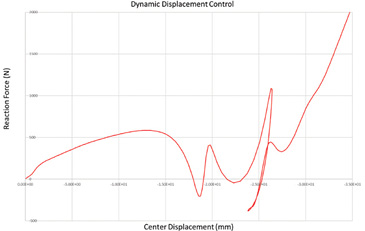
The plot tracks the entry to the snap-through and the recovery to the stable configuration. It’s interesting that the snap-through is now responding dynamically with an overswing of the plate producing an oscillation before contact is re-established. The strange shape of the curve within this period is due to the changing phase between the center deflection and the net reaction force. Plotting displacement and reaction force independently against time show normal oscillatory behavior.

ANSYS Workbench allowed me to explore the snap-through benchmark in greater depth. I have not used classic ANSYS for many years, but found the Workbench environment allowed me to quickly get up to speed again. The workflow made repetitive tasks, such as investigating the influence of non-linear settings, straightforward. The ability to quickly plot, review and paste to Excel allowed a large amount of data to be investigated efficiently.

The Project Schematic window helped me organize the different analyses used in the investigation: displacement control, load control, contact control and dynamic control, from one central point, rather than a series of separate databases. 

Tony Abbey has created a non-linear e-learning class that is presented in partnership with NAFEMS. Check out the content at goo.gl/otYmDY.

More Ansys Coverage