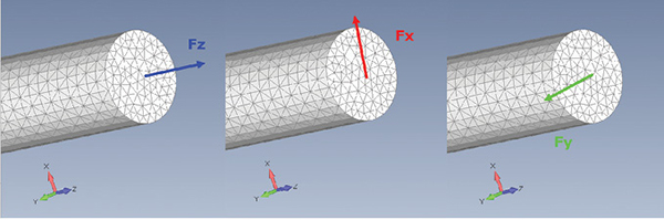
Fig. 1: Three separate loads applied to end of rod. Images courtesy of Tony Abbey.


Latest News
November 1, 2019
Editor’s Note: Tony Abbey provides live e-Learning courses, FEA consulting and mentoring. Contact tony@fetraining.com for details, or visit his website.
Earlier this year, I presented a short course on interpreting stresses at the NAFEMS World Congress in Quebec. The material was largely drawn from my series of articles in DE (March, May and July 2016; see links at end of article).
At the beginning of the session, I explained why I preferred to start a discussion on stress by looking at force vectors. I was interrupted by a gentleman who made it clear he did not understand—or even believe—what I was talking about. It turns out he had a computational fluid dynamics (CFD) background, had never dealt with stress and considered it was trivial to deal with!
That got me thinking about revisiting the topic. I decided to build a few simple finite element analysis (FEA) models to explain stress in context, and also expand on the role of shear stress. Shear stress is something that puzzles a lot of engineers and took me many years to figure out.
Force is a Simple Vector
Fig. 1 shows the end of a rod that is loaded with three separate load cases: Fz, axial force in z, Fx shear force in x and Fy shear force in y.
The relationship between the force vector and the plane it acts on defines the sense of the force. The common loaded plane is the XY plane (or in a contracted notation, referred to as the Z normal plane). I have color-coded the forces with the format used in the FEA coordinate system symbol seen in the figure.
The forces can be combined to form new loadings, and a vector can describe the resultant. Fig. 2 shows some examples of load combinations. The contributions of the axial and two shear forces are very easily seen.
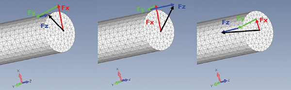
In each case, the resultant force is shown as a black arrow.
The force notation used in Figs. 1 and 2 is a bit “wooly,” or arbitrary, and there is no clear distinction between direct and shear forces. You have to rely on the descriptions already noted!
In previous articles, I described the “force cube.” For our purposes, I have modified the diagram in the figure from those articles to align with the specific loading plane and loading direction across the rod section. I have also labeled direct forces with blue and shear forces with red (not to be confused now with the previous colors.)
This is formalizing the force notation based on the plane the force is acting normal to, and the direction of the force. This allows us to clearly differentiate between direct and shear forces. The first force index is the plane normal; the second index is the force direction.
In this case, the axial load in Figs. 1 and 2 is Fzz, simplified to Fz. The vertical shear force loosely described in Figs. 1 and 2 as Fx, is more precisely defined as Fzx. It is in the plane normal to z and is pointing in the x direction. The lateral shear force, described as Fy, is properly defined now as Fzy. It is in the z normal plane, but points in the y direction.
Stress is Not a Simple Vector
As a non-mathematician, I can understand why this heading may leave you cold. What does it mean? Why is it important? This is why I like to use force to start the discussion on stress.
If we imagine the forces are now internally applied to a very tiny cube of material deep inside the rod, we can imagine the stress state does not change across any of the faces. A “stress cube” can be drawn, where each stress is just the force/area in the limit. Fig. 3 shows the stress cube, which corresponds exactly to the force cube.
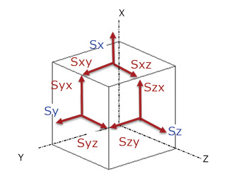
Using this diagram, imagine we have an axial stress Sz and a shear stress Szx. Both are being applied to the z normal face, but I cannot combine them as a vector with the simple chain rule I used with forces. I have to describe the stress state in terms of the component stresses Sz and Szx. And therein lies the difficulty with stresses; it is difficult to describe, or indeed visualize, a combined stress state.
We have to resort to other methods to try to understand the importance of the stress in terms of its effect on strength. One of the most common methods is to use the von Mises equivalent stress. This applies weighting to shear terms and combines all the stress contributions. In the case already mentioned, we add (Sz)^2 and (3*Szx)^2 and then take the square root. The factor of 3 on shear stress inside the square root is based on von Mises theory and ties up very well with the experimental evidence that yield strength in shear is less than yield strength in tension.
Examples Using FEA
First, let’s apply the axial force Fz to the rod. The value is 31,153 lbf. The cross-sectional area, A, is 3.14 inches ^ 2. The stress should be constant across the section at 9,921 psi. The FEA result is 9,928 psi due to small errors in the mesh cross-sectional area.
It would seem that there is a simple relationship between the axial load and the axial stress. However, this is a stress state, not a vector, and we can look at it in different ways. For example, the commonly used Tresca failure theory uses the maximum shear stress component from a uniaxial tensile test. How can this be? It is a tension test!
In fact, we can look at the small stress cube, but use it to develop force components, which can be balanced, as they are vectors. The procedure is shown in Fig. 4.
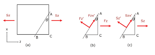
Fig. 4(a) describes the stress state, looking at the side of the cube. A section is cut at an angle theta. A force diagram is shown in Fig. 4(b). The forces are related to the stresses shown in Fig. 4(c) by the cut areas (assuming a unit depth in y).
Fz = Sz*AC
Fz’=Sz’*AB
Fzx’= Szx’*AB
The prime symbol (‘) relates to the new coordinate system after rotation by theta.
Using force balances in Fig. 6(b):
Horizontally; Fz’=Fz cos(theta) - equation (1)
Vertically; Fzx’=Fz sin(theta) - equation (2)
From the geometry AC = AB cos(theta)
Hence in equation (1); Sz’*AB = Sz*AC cos(theta) = Sz* AB cos(theta) cos(theta)
Direct stress, Sz’ = Sz* cos^2(theta)
Hence in equation (2); Szx’*AB = Sz*AC sin(theta) = Sz* AB cos(theta) sin(theta)
Shear stress, Szx’ = Sz* cos(theta) sin(theta)
This relationship is shown in Fig. 5.
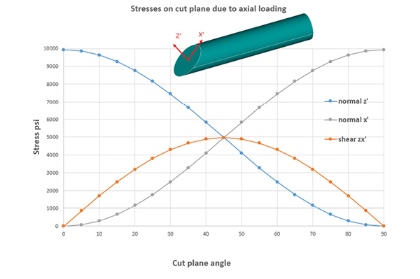
At zero cut plane angle, all the Sz’ stress is axial (being aligned with z direction). Rotating to 45º gives the maximum shear, Szx’. The balancing direct stress in the local x’ direction can be calculated in the same way, but using a cut plane rotated 90º.
We can check out these results by using the model, as shown in Fig. 6.
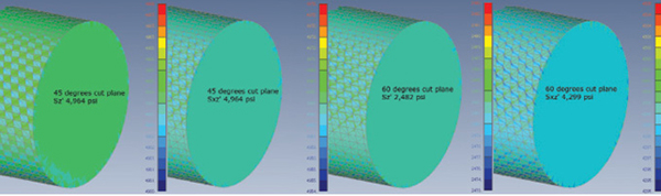
I created two local coordinate systems in the model, rotated at 45º and 60º about the y axis. In the post-processor, I transformed the stresses to each local coordinate system in turn. The stresses are constant across the section, with very small perturbations due to numerical drift. The stresses in Fig. 6 agree with the theory, using the graph shown in Fig. 5.
The shear stress is labeled as Sxz’ in Fig. 6(b) and 6(c). However, remembering the index notation, this should mean it is acting in the x (normal) plane shearing in the z’ direction. Surely the stress should be labeled Szx’ as it is in the z’ plane and acts in the x’ direction! Check Fig. 3 for the answer; Szx is equal to Sxz. The post-processor rather lazily just uses one term to describe both equivalent shear stresses. Though it would take an intensive and complicated effort to automate this.
For each of the coordinate system transformations used (0º, 45º, 90º), the von Mises stress was found to be identical. This is because we only have one stress state due to the axial loading. This is reduced to a single scalar value with the von Mises equation. The cut plane—or transformation angle—just provides a different way of looking at the same stress state.
The 45º plane is interesting, because it provides the biggest shear component, Sxz’. It is numerically equal to half the axial tensile stress Sz at a zero cut plane. If a material is weaker in shear compared to tension by a factor greater than 0.5, then a shear failure may occur in a tensile test. If the axial load is compressive, then some materials exhibit a shear failure on a 45º slip plane. In mild steel Lüders lines or slip lines can sometimes be seen at 45º in a tensile test (see vimeo.com/4586024). In general, the material behavior can get very complex, but the point is that shear components are lurking in the stress state under axial loading.
Shear Loading
In the next example, I applied a force of 31,153 lbf in the x direction at the end of the rod. This then acts like a cantilever beam with a constant shear force and a linearly increasing bending moment. The stress state at a position along the rod is shown in Fig. 7.
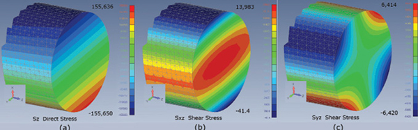
The direct stress Sz, which is due to bending, is shown in Fig. 7(a). As expected, we have maximum at the top, tension surface and minimum at the bottom compression surface. The values are equal and opposite with a small numerical drift.
The shear distribution through the depth of a solid section is parabolic. The shears at the extreme top and bottom surfaces must be zero, and build to a maximum at the neutral axis. Basic shear theory calculates the maximum shear stress to be 4/3 of the nominal shear stress for a circular cross-section. The nominal value is 31,153/3.14 = 9,921 psi. The theoretical maximum is 13,228 psi. The FEA maximum value is higher at 13,983 psi.
What’s interesting is that the basic theory assumes that shear variation is only a function of depth. This would imply non-zero tangential shears building up at the periphery of the rod, below the top and bottom positions. The plot in Fig. 7(b) is not in fact a function of depth alone. Popov 1 suggests that the manual calculation gives the correct vertical component of shear stress, but that there is another horizontal component missing. Fig. 7(c) shows the missing component Syz, which balances the shear state to give zero “out of surface” shear at the free edges. The maximum shear stress is assumed to be within 5% of the simple theory, which seems to be the case here.
Fig. 8 shows a further attempt to describe the shear state, using a cylindrical coordinate system to look at radial and hoop components.
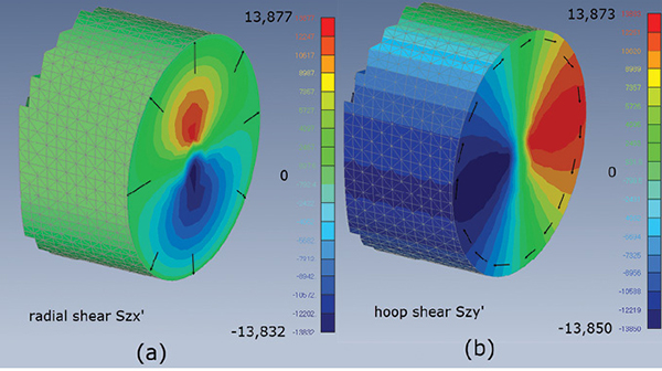
In Fig. 8(a) the radial stresses are zero at the outside wall—and this is the improvement over the manual calculation. Fig. 8(b) shows the shear flow around the outside wall, being a maximum at the neutral axis and decaying to zero at the top and bottom. The shear stress sign change is due to left and right edges acting positive upwards, that is, anticlockwise, then clockwise.
Unfortunately, using von Mises stress will not help give a picture of the shear stress contributions. Remember Fig. 7(a)? This shows that the axial stress Sz dominates. This will be included in the von Mises calculation and obscure the shear stress terms. It may be that a macro could be written to exclude the direct stress in producing a “shear only” pseudo von Mises stress.
Torsional Stresses
A torsional load of 100,000 lbf in. was applied at the end of the bar. From basic calculations, the torsional constant, J, is given by:
J = pi*D^4/32, where D is the diameter.
The torsional constant with D of 2.0 inches is 1.571 in^4. The maximum distance from the center of rotation, c is D/2. The peak shear stress due to torsion is given by:
S,shear,max = TJ/c
The maximum shear stress is 63,662 psi. The FEA results are shown in Fig. 9.
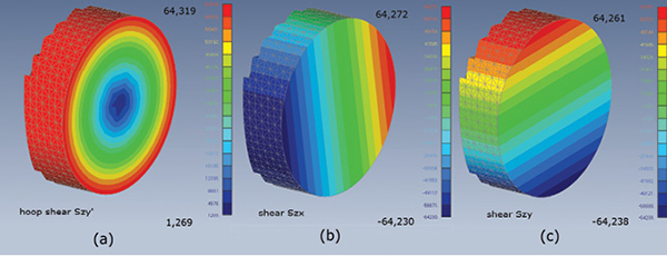
Fig. 9(a) shows the shear stress in the hoop direction, using the basic cylindrical coordinate system. This is the most logical way to plot torsional shear as it flows in this sense. The maximum value from FEA is 64,319 psi, compared to 63,662 psi in the manual calculation. The error is probably a combination of errors in effective diameter due to meshing of the circular cross-section and numerical drift in the FEA method. The stress distribution is also distorted away from purely concentric rings of constant stress at the center of the section.
Figs. 9(b) and 9(c) show the component shear stresses in the basic cartesian coordinate system. This is a similar issue to that found previously: shear stress components have to be combined to achieve meaningful results. In this case the shear stresses in the cylindrical hoop direction, Szy’ completely define the stress state as shown in Fig. 9(a). The radial component, Szx’ is zero.
A further interesting reflection on manual calculation methods is that it is extremely difficult to predict shear stresses under combined loadings, particularly with arbitrary cross-sections. This is where FEA can give a full distribution—we just have to figure out how to visualize it!
Conclusion
Stress is a difficult quantity to describe and interpret. Considering contributing force vectors in parallel may help visualize stress states. Using simple FEA models of configurations that have known classical solutions can be a big help.
However, even then analysts need care to interpret the stress components, particularly in shear. We also have the issue that some problems such as shear stress in a circular section due to shear loading are simplified in classical solutions.
I suggest trying a few other sections using this approach—perhaps an I-beam or thick box girder will show similar interesting results!
Reference
1 E. P. Popov. Mechanics of Materials. 2nd ed. Upper Saddle River, NJ: Prentice Hall, 1976.
Previous DE articles by Tony on FEA
Subscribe to our FREE magazine, FREE email newsletters or both!
Latest News
About the Author
Tony Abbey is a consultant analyst with his own company, FETraining. He also works as training manager for NAFEMS, responsible for developing and implementing training classes, including e-learning classes. Send e-mail about this article to DE-Editors@digitaleng.news.
Follow DE