Fig. 14: Tool tips on half model.


Latest News
March 1, 2018
Editor’s Note: Tony Abbey teaches both live and e-Learning classes for NAFEMS. He also provides FEA consulting and mentoring. Contact tony@fetraining.com for details.
We previously carried out trial meshing on the geometry in part 1 of this article. Now it’s time to set up the production mesh. I split the geometry into two bodies to force nodes to be created on the centerline datum plane. I set the FEMAP mesh control option to merge nodes on common geometric faces. Otherwise, the FEA model would have a split between the two meshed bodies.
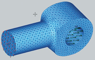 Fig. 1: Initial mesh.
I am using tetrahedral elements because the geometry is an arbitrary shape. FEMAP supports hexahedral elements, but it would take a lot of work to prepare the geometry for a hexahedral mesh. I have used the default global element size, and the resulting mesh is shown in Fig. 1.
The mesh looks smooth in the figure, but it is inadequate around the blend region between the shaft and the end fitting and through the radial depth of the end fitting-bearing surface.
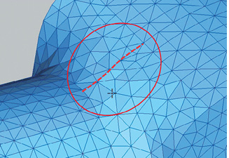 Fig. 2: Poor initial mesh.
Fig. 2 shows the blend region in more detail. We are anticipating high stress concentrations around here, and there are not enough elements to produce a good result.
This is a typical starting point in any meshing task, and I use the FEMAP tools to improve the situation. There are a hierarchy of meshing controls within FEMAP.
The top level is the default element size, which is based on overall geometry dimensions. The next level controls the size of elements within a solid body using the body edge curves. The number of elements along each edge curve is used as a guide. There is a default number of elements applied to each edge curve. Using this default results in a similar mesh to that created with the default element size. The default sizes tend to be very conservative and result in a coarse mesh that can be viewed as being adequate for a Normal Modes analysis but usually unacceptable for a strength analysis. The objective is to selectively increase the number of elements along key edge curves to improve the mesh within the body.
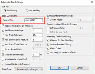 Fig. 3: Meshing controls.
There are a rich set of mesh controls, as shown in Fig. 3. These include the rate at which element size grows away from the smallest elements (finest mesh) and curvature-based meshing. It is a good idea to practice on a variety of simple CAD geometry models to get the feel for how these tools interact. Meshing is an art, not a science, and it takes practice.
To attempt to heal poor geometry, it is possible to suppress short edges and eliminate small features. By default, adjacent surfaces, such as in the split bodies in the tie-rod geometry, will have matching meshes, ready for merging.
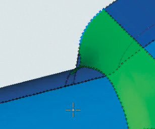 Fig. 4: Preview of mesh.
The emphasis with any preprocessor is to set up a meshing strategy and then experiment. I typically try at least a dozen or more meshing variations before I am satisfied. FEMAP greatly assists here by providing a meshing preview. Fig. 4 shows the edge mesh size visualization as a series of dots. The preview can be easily switched on and off from the toolbar.
I have set this to a very fine value, as a demonstrator. This ability to preview without committing the meshing process speeds up the meshing development. In this case the mesh is so fine that the mesh would take a long time to complete and the element count would be way too high.
It is a good idea to get a feel for a “safe” lower limit on element size. If the mesh is too fine it may take a long time to complete, or even stall the preprocessor.
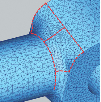 Fig. 5: Improved mesh.
The strategy I adopted for the blend region between the tie rod shaft and end fitting is to control the mesh size along the key edges, as shown in Fig. 5. I had an initial idea of the number of elements needed on each of these edges. By experimenting with the numbers, I am able to get a reasonable looking mesh.
Progressively increasing the number of elements on edge curves to produce a series of meshes can be a frustrating experience. Mesh quality can jump up and down with no apparent reason. The meshing process is essentially a pattern generator and is very unpredictable, which is why experimentation is key.
I normally recommend approaching each meshing task with a time limit in mind. Allow 30 minutes to produce the best-looking mesh in each critical region. Fig. 5 shows such an effort after about 30 minutes of work.
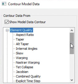 Fig. 6: Mesh quality controls.
I have talked about “good-looking” meshes, but we need a more objective assessment of element quality. FEMAP has a range of mesh quality plot options, as shown in Fig. 6. The two I use most from this list are the Jacobian and the Tet collapse. Other analysts may have their own favorite metrics.
It is difficult to give advice on what values to use for these two parameters, as each one is solver and element type dependent. I recommend setting up a series of simple geometric benchmarks, such as a solid plate with a hole in it. These can then be meshed and analyzed to correlate stress results with mesh quality. Fig. 7 shows the Tet collapse element quality plot. In my case I used a value of 4.0 as the upper bound on Tet collapse, from inspection.
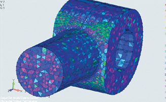 Fig. 7: Tet collapse check.
It is difficult to see the distribution of “rogue” elements that exceed the limit, within the element fill plot for 3D solid structures. One of the control options within the quality contour plotting is to set up a group containing all elements that have exceeded a certain level. In Fig. 8, I have plotted this group. I have also included a wireframe plot of the tie rod geometry.
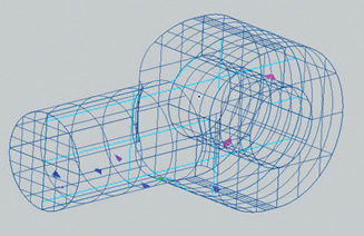 Fig. 8: Rogue elements.
As an aside, groups are a useful FEMAP functionality. Groups can consist of sets of entities of any mixture. In my case I had a group with rogue elements and solid geometry. Groups can be used to focus on specific model regions, for example, one of the solid bodies and its elements and nodes. They also can be used as selection tools. I set up the key meshing curves shown in Fig. 5 as a group to allow easy picking. I would recommend that any newcomer to FEMAP practice using groups, as they will underpin many other operations.
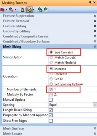 Fig. 9: Mesh toolbox controls.
An alternative to the manual mesh updating strategy shown so far is to use the FEMAP meshing toolbox. This collection of meshing methods has been developed over the last few years and includes an interactive meshing capability. The controls are shown in Fig. 9. I have set up interactive meshing action using edge control, adding one element to each edge when I run the tool. I can then cycle through and increment that element count automatically.
When using the toolbox, as the mesh is updated, the element quality also updates. Fig. 10 shows a montage of mesh quality plots as I step through a range of meshes with increasing fidelity. The increasing number of elements runs from top left to bottom right in the figure. The plots show the mesh on the inside face of the fitting, another critical region. The random nature of the meshing operation is clearly shown. One or two configurations are rejected because of “rogue” elements appearing. The ability to experiment and quantify the mesh quality helps greatly in the search for the “perfect mesh.” FEMAP allows for a large number of undo and redo operations, so it is easy to step backward and forward to make your pick of the best mesh.
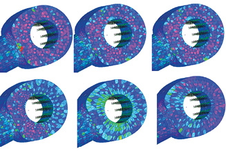 Fig. 10: Montage of mesh quality results.
Once meshing is complete, it’s time to set up the NX NASTRAN analysis. Fig. 11 shows the analysis control panel. I’m using a static analysis here, but FEMAP supports a full range of analysis available within NASTRAN, including dynamics and non-linear. I’ve picked the NX NASTRAN solver bundled with FEMAP in my installation. There are many solvers to select, including MSC/MD Nastran, ANSYS, ABAQUS, LS-DYNA etc. This is a reminder that FEMAP started life as a solver neutral pre- and post-processor. If you are using multiple solvers on an FEA project, this can be a useful attribute.
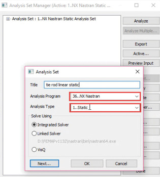 Fig. 11: Analysis setup.
On launching the analysis, an Analysis Monitor pane pops open, as shown in Fig. 12. This allows users to inspect the output text files that contain runtime diagnostics and output data summary. It also tracks the progress of the solver. This is particularly useful in long-running analyses. It also allows monitoring of convergence in non-linear analyses.
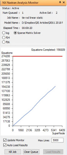 Fig. 12: Analysis Monitor.
Once the analysis is complete, the results are loaded into the FEMAP database and the post-processing toolbar becomes live. The default output quantities are deformation and von Mises stresses. The stress contour plot is shown in Fig. 13.
The default settings for stress plots in the post-processor show a continuous color rendering and use nodal averaging of stresses. I recommend these are changed to, respectively, level colors, to give hard edges to the contours and switching nodal stress averaging off. Stress averaging can hide poor stress distributions and artificially lower the peak stress values.
The highest stresses in the tie rod are along the center line at the end fitting bearing face. This is where the geometric split in the model is useful, as it allows for plotting of the stresses accurately on the cut plane. This is shown in Fig. 14. FEMAP does have section slice controls that allow visualization of stresses in an arbitrary plane. However, these will always be interpolated by the post-processor, whereas geometry slicing guarantees better accuracy on the plane.
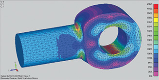 Fig. 13: von Mises stress.
Figure 14 also shows the use of tooltips. Any element can be selected, and a text box produced on the plot showing the values of the contour quantity selected. Probing in specific regions is then easily achieved.
Finally, Fig. 15 shows the deformation of the tie rod. This can be scaled to help visualization. Too small a scale, and it’s difficult to see the sense of the deformation. Too large a scale can be equally confusing. Here, I have augmented the deformation plot by also plotting a translucent image of the geometry. Other techniques in FEMAP include a wireframe outline of the undeformed mesh.
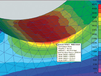 Fig. 14: Tool tips on half model.
Deep, but Daunting
FEMAP with NX Nastran is a mature product, providing a rich set of features to carry out mainstream FEA. For a new user, the breadth and depth of functionality can be daunting. However, once an initial subset is mastered, aided by the use of customized toolbars, the “toolbox” can be logically expanded to achieve a high level of productivity.
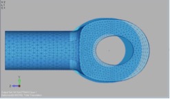 Fig. 15: Deformation.
Key aspects of FEMAP to focus on initially include picking methods, adaptive dialog boxes, adaptive Method menus and groups.
A set of five supporting videos are available for view at digitaleng.news/de/femapnx2. The geometry files for the part are located at digitaleng.news/de/nxgeometry.
Subscribe to our FREE magazine, FREE email newsletters or both!
Latest News
About the Author
Tony Abbey is a consultant analyst with his own company, FETraining. He also works as training manager for NAFEMS, responsible for developing and implementing training classes, including e-learning classes. Send e-mail about this article to DE-Editors@digitaleng.news.
Follow DE