
Latest News
June 1, 2018
SOLIDWORKS Simulation is an add-in to the SOLIDWORKS program from Dassault Systèmes. It provides a finite element analysis (FEA) capability within the traditional CAD environment. This is attractive to design engineers and others who are familiar with the SOLIDWORKS user interface.
A wide range of FEA solutions are available, from linear static to non-linear dynamic analysis. However, a potential purchaser needs to work closely with their SOLIDWORKS reseller to define the precise range of solution capabilities needed. The segmentation of the CAD functionality interleaved with the FEA functionality can be very confusing.
The origins of the FEA solution within SOLIDWORKS stem from the COSMOS FEA solver, a different solver from the advanced nonlinear Abaqus solver found within the Dassault Systèmes SIMULIA product family.
The Aircraft Keel Project
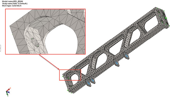
The FEA task in this review is to carry out a static analysis study of the aircraft keel section shown in Fig. 1. In part one of this overview, I focus on the initial setup and the solid meshing controls.
The keel section is on the lower centerline of a combat aircraft fuselage. It transmits undercarriage loads into the fuselage. It also provides a load path through the lower fuselage section in overall bending and torsion loading due to maneuvers. The geometry has been created in SOLIDWORKS. Many of the smaller fillet radii have been defeatured in preparation.
The Simulation add-in has been invoked in Fig. 1. Two new tabs appear in the CommandManager area; the Simulation tab and the Analysis Preparation tab. The Simulation tools are shown. The Study Advisor icon is selected, and a new Simulation Study is set up. This is a static analysis study; undercarriage_case1.
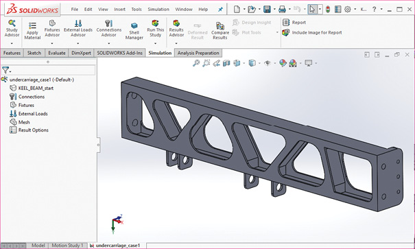
Multiple studies can be created in a SOLIDWORKS file and each will have a tab on the bottom of the screen. To switch between the simulation study and the geometry model, click on the Study or the Model tab. The Analysis Preparation tab contains a useful subset of geometry tools to manipulate the geometry ready for analysis.
The feature tree in the left-side panel contains icons that give access to required FEA entities. Right mouse-clicking on the top Study icon provides a menu that includes the analysis Properties selection. Fig. 2 shows the resultant dialog box.
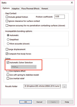
Within the highlighted Solver Selection drop-down are a range of FEA solver options, including Direct and Iterative solvers. The optimum choice of solvers is complex, dependent on solution type, model size and available system memory. I checked the Automatic Solver Selection option. This adopts the best method based on the characteristics noted. I recommend reviewing the documentation carefully and carrying out benchmarks to decide which solver setting is most applicable. There can be big differences in runtime, so time spent tuning will be worthwhile.
Standard Mesh Control
The mesh icon in Fig. 1 pops up a dialog box, as shown in Fig. 3 on the left, from which I selected the Standard mesh method. The mesh density is controlled with a slider bar, or by inputting two parameters: maximum and minimum element size. The default, specific to my model, is a medium density setting with maximum and minimum element sizes set to 0.782 in. and 0.039 in. The 20:1 ratio is the default. It is important to know your critical geometry dimensions and the implications within the settings. Fig. 4 shows the overall mesh and the local mesh around the critical stress area.
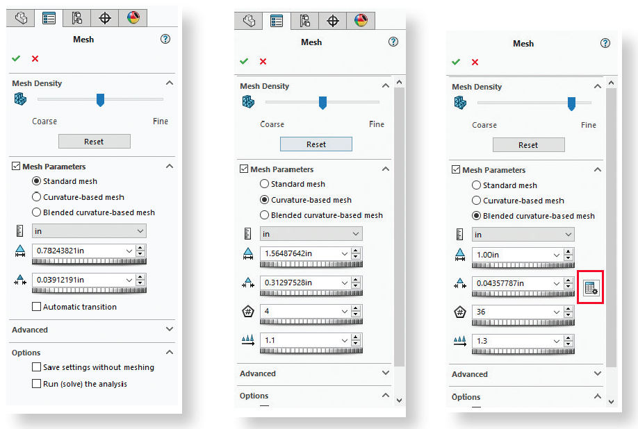
Fig. 3: Standard (left), curvature (center) and blended-curvature based options in the Meshing menu. Images courtesy of Tony Abbey.
I ran an exploratory analysis (not shown) to confirm the high stress areas. These are the fillet radii seen in the inset of Fig. 4, which need a fine mesh. The adjacent bolt hole needs a coarser mesh and is typical of the rest of the structure.
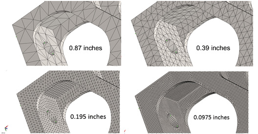
The bolt hole periphery is 3.14 in. (0.5-in. radius). The fillet periphery is 1.57 in. (1.0-in. radius). The default maximum element size forces two elements around the fillet radius, nine around the bolt hole. The mesh shown in Fig. 4 is generally too coarse, and far too coarse at the fillet. The model has 61,701 degrees of freedom (DOF).
The “Fine” setting gives maximum and minimum element sizes of 0.39 in. and 0.019 in. Now four elements are forced around the fillet and nine around the bolt hole. This mesh is shown at top right in Fig. 4. The general mesh size is acceptable now, but the fillet is still far too coarse. The model has 210,501 DOF.
I have progressively halved maximum element size by manually setting to 0.195 and 0.0975 in., as shown in Fig. 5, bottom left and right. The model sizes are 1,234,647 DOF and 7,687,593 DOF. For a converged stress at the fillet, the local mesh size needs to be around 0.0975 in., as shown in the last model, but this is clearly not an acceptable solution. My desktop with 64GB RAM hit a wall here and took 23 minutes to mesh!
This academic exercise shows the need for alternative meshing strategies, and SOLIDWORKS offers three approaches: curvature-based meshing, local mesh control and adaptive meshing. The first two methods are based on user-defined controls. Adaptive meshing uses a series of automatically created analyses that update the mesh to minimize stress jumps between adjacent elements. The program seeks out stress concentrations and refines the local mesh.
Curvature-Based Meshing
In the curvature-based option of the mesh dialog box (Fig 3, center), the slider bar controls maximum and minimum element size, as before. The default element size is coarser. The key parameter is the minimum number of elements around a circle (curvature control), shown by the pentagon-shaped icon. The range is between 4 (default) and 36 (maximum).
The default curvature setting of 4 gives a very coarse mesh of 56,097 DOF, as shown in Fig. 6.
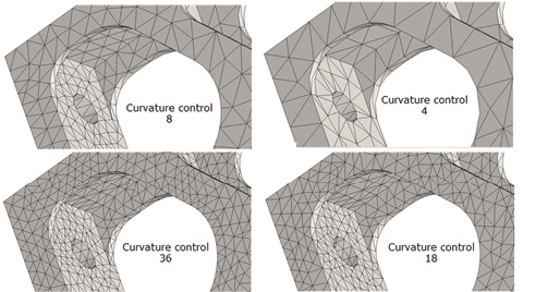
Successive curvature controls of 8:18:36 are also shown in Fig. 3, center. The model sizes are 106,563 DOF, 195,252 DOF, and 252,768 DOF. There is little difference in the meshes beyond curvature control 18. The fillet and bolt hole element numbers are stuck, because the minimum element size has not been changed. The fillet periphery is 1.57 in., the minimum element size is 0.312 in., hence five elements are allowed. Similar math shows the limit around the bolt hole of 10 elements. Without this insight, use of the curvature-based meshing can be frustrating, as it appears to stall.
If we back-calculate, nine elements around the 90° fillet give a minimum element size of 1.57/9 = 0.174 in. This is the maximum in curvature-based meshing control (36 around a full circle). Using a smaller element size does not allow for a higher number.
Using these settings, a reasonable mesh is created, shown in Fig. 7, labeled Growth Rate 1.1. The model has 732,612 DOF. The maximum element size of 1.56 in. is the default, but the largest elements in the figure are much smaller than that. It would be useful to be able to further coarsen the mesh away from the fillet. The clue is the Growth Rate parameter, shown as a series of triangles in the menu. The value of 1.1 is the size multiplier on each successive element layer. A value of 1.1 gives a very slow growth rate from the fillet. The effect of growth rate is shown in Fig. 7.

Setting the value to 1.3 gives a useful gradation from the fillet to the edge and a model with 411,282 DOF. Over 300,000 DOF are saved. The next mesh at Growth Rate of 1.5 shows how sensitive this parameter is, since the model size has dropped to 287,964 DOF. Finally, a setting of 2.0 on Growth Rate gives 173,685 DOF. The fillet local mesh size has remained constant during these meshing runs.
The keel structure is relatively “narrow” in all places, so the Growth Rate does not have enough element rows to achieve the maximum element size of 1.56 in. The maximum element size is redundant here, but in a “wide” structure where many element rows exist, away from controlling curvature-based features, the mesh can coarsen to the target value.
To sum up the Curvature-based mesh strategy:
1. Select critical curved features and calculate the element size for 36 elements in a 360º circle.
2. Set this as minimum element size.
3. Set growth rate to 1.5.
4. Set the largest target element size in the coarse mesh region.
5. Adjust the Growth Rate until you find a gradation you like.
Blended Curvature-Based Meshing
This is an automated version of the curvature-based meshing. The dialog box is shown in Fig. 3, right.
The highlighted button in the dialog box activates a calculator that finds the smallest curvature-based feature in the model. The blended curvature-based smallest element size is 0.0435 in., because of 0.25-in. radius bolt holes that are present. The other parameters remain the same, using settings from the previous exercise. Fig. 8 shows the resultant mesh.
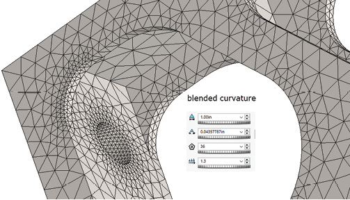
Interestingly, the blended mesh overrides the limit of 36 elements around a circle, using the new smaller minimum for all curved surfaces! This produces a good mesh around the fillet—but is overkill in other non-critical curved regions. The model has 674,685 DOF.
This method could be used as an additional “step 6,” after normal curvature-based meshing settings are established. The blended mesh minimum element size, entered manually, would “nudge” up the number of elements around key features.
Local Mesh Controls
After curvature-based meshing, the fillet has reached its limiting size. This is frustrating as we need a finer mesh at the fillet. Local mesh control now plays a key role.
Right mouse-clicking on the mesh icon allows Apply Mesh Control to be selected. Fig. 9 shows the menu and the fillet surfaces chosen.
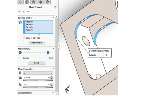
I have halved the “stalled” fillet mesh size. The resultant mesh is shown in Fig. 10.
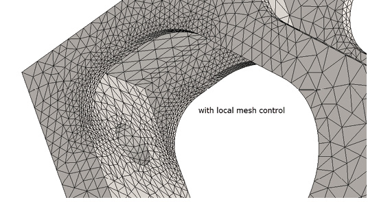
The local mesh control is highly selective. It allows good mesh refinement at the fillet region, while keeping the model size to 385,899 DOF.
Individual mesh controls can be set. Using these as fine control adjustments on a sound baseline mesh provides a powerful technique.
Conclusion
The solid meshing controls in SOLIDWORKS Simulation allow very good mesh control. However, there is a great deal of interaction between parameter settings. To avoid frustration, I recommend exploring the options with simple geometry to develop a consistent workflow.
In part two of this SOLIDWORKS Simulation walkthrough, I will review loads and boundary conditions and then focus on the post-processing options.
More Dassault Systemes Coverage

For More Info
Subscribe to our FREE magazine, FREE email newsletters or both!
Latest News
About the Author
Tony Abbey is a consultant analyst with his own company, FETraining. He also works as training manager for NAFEMS, responsible for developing and implementing training classes, including e-learning classes. Send e-mail about this article to DE-Editors@digitaleng.news.
Follow DE